
Building Newmark’s influence chart
April 26, 2024 at 2:03 PM by Dr. Drang
After writing the last post, I decided to do the calculations necessary to make Newmark’s influence chart.

I started with the Boussinesq equation:
If you compare this with the formula I gave last time, you’ll see that I’ve deleted the negative sign. That’s because tensile stresses seldom arise in soil mechanics, so the convention is to take compressive stresses as positive.
This is a solution to the elasticity equations in cylindrical coordinates, , where the origin of the coordinate system is at the point on the surface where the load is applied. Notice that there’s a circular symmetry to the solution— is independent of the angle .
This symmetry has an interesting and very useful consequence. We can move the origin of the coordinate system to the point on the surface above the point at which we are calculating the stress, and the formula for will remain the same. We’ll use this to figure out the stress1 associated with a distributed load.
Because Newmark has made his chart as a series of rings split into sectors, we’re going to calculate the stress due to a uniform distributed load, , acting over one of these sectors. The two radii that bound the sector are and , and the two angles that bound the sector are and .
 With this loaded area defined, we can write the resulting stress as
Because the integrand doesn’t contain , that part of the integral will result in a term, which we’ll call . That term, along with the constants, can be brought outside the integral over :
If there were an analytical solution to this integral, we’d be in business, but I don’t think there is. I gave the problem to Mathematica, and it thought for over five minutes without coming up with an answer before I stopped it. So we’re going to have to use numerical integration, which means it’s time to nondimensionalize the equation.
First, we note that is nondimensional. This fits in with Newmark’s scheme, because this is what he calls the influence value (see the lower right corner of the chart). So we know this term is going to be 0.001.
Second, we see that Newmark split each ring into an integral number of sectors. The number of sectors isn’t the same for each ring, but we can always say that
where is a positive integer. Therefore,
Finally, we note that Newmark scales the radii of the rings by the depth, . So we’ll define a new variable, , and rewrite the integral using this change of variable. We see that
and (this may not be as obvious, but you can check it)
So with these substitutions, we get
Hey, look! The ’s all cancel out, and we’re left with
Note that all the terms in this equation are pure numbers; none of them have any units, like feet or meters or pounds. That’s what I meant by “nondimensionalize.”
So now all we have to do is find a sequence of values for and that will solve this equation for the appropriate value of . Starting at the origin of the chart, we know that and (you may have to zoom in to see that), and we can solve for . Then for the next ring, we use the previously calculated value of as our new value for and set . This continues on for all 25 rings in the chart.
The box below should contain the Mathematica notebook I used to do the calculations. If it’s empty, that means the Wolfram Cloud is being slow and stubborn, so you might have better luck following this link. Or not. I don’t have a lot of experience with the Wolfram Cloud, but so far I’ve noticed that it isn’t as responsive as the documentation would have you believe.
Whether you have any experience with Mathematica or not, I think the logic of the notebook is relatively easy to follow. For each pass through the Do loop, we’re calculating a new upper limit for the numerical integral that solves the equation. That value is then appended to the list of radii and gets used as the lower limit of the numerical integration during the next loop. Finally, the ring thicknesses are calculated by subtraction.
The results are summarized in this table:
| Ring | Sectors | Outer radius | Thickness |
|---|---|---|---|
| 1 | 8 | 0.07327 | 0.07327 |
| 2 | 16 | 0.12778 | 0.05450 |
| 3 | 24 | 0.18259 | 0.05481 |
| 4 | 24 | 0.22600 | 0.04342 |
| 5 | 24 | 0.26382 | 0.03781 |
| 6 | 48 | 0.33048 | 0.06667 |
| 7 | 48 | 0.39080 | 0.06032 |
| 8 | 48 | 0.44807 | 0.05727 |
| 9 | 48 | 0.50413 | 0.05606 |
| 10 | 48 | 0.56025 | 0.05612 |
| 11 | 48 | 0.61747 | 0.05723 |
| 12 | 48 | 0.67678 | 0.05931 |
| 13 | 48 | 0.73921 | 0.06243 |
| 14 | 48 | 0.80596 | 0.06675 |
| 15 | 48 | 0.87854 | 0.07258 |
| 16 | 48 | 0.95895 | 0.08041 |
| 17 | 48 | 1.05003 | 0.09108 |
| 18 | 48 | 1.15606 | 0.10603 |
| 19 | 48 | 1.28396 | 0.12790 |
| 20 | 48 | 1.44608 | 0.16213 |
| 21 | 48 | 1.66772 | 0.22164 |
| 22 | 48 | 2.01358 | 0.34586 |
| 23 | 32 | 2.41493 | 0.40135 |
| 24 | 32 | 3.31945 | 0.90452 |
| 25 | 16 | 4.89898 | 1.57953 |
The inner radius of each ring is the outer radius of the ring before it. The exception is the first ring; recall that its inner radius is zero.
My first thought after running out these calculations was to check the numbers against measurements I could take from the chart. They were pretty close. Not perfect, but typically within a couple of percent. I couldn’t really expect any better, as the chart (which is a page from this PDF) wasn’t scanned at a particularly high resolution (only 150 dpi), and it wasn’t perfectly aligned with the scanner (the horizontal axis isn’t quite horizontal).
But would Newmark include a chart without giving the data necessary for readers to reproduce it? Of course not. In the appendix is a table of values for making all the various influence charts discussed in the paper.2 Here’s an excerpt from the table that shows the ring radii for the vertical pressure influence chart.

It’s the third column, which gives the radius as a fraction of the depth, , that we can compare to the “Outer radius” column in the table above. As you can see, all the numbers match to three decimal places except the one for the 24th ring. Newmark shows 3.315, when the value should be 3.319. Should we blame the student who did the calculations, noted in the acknowledgments as Harold Crate? Should we blame the unacknowledged secretary who typed up Crate’s calculations? No, we have to blame Nate Newmark himself—after all, he’s the guy whose name is mentioned in all the soil mechanics textbooks.
-
If you haven’t noticed yet, I’m using the words, stress and pressure interchangeably because for this problem they are the same when I’m talking about what’s going on at depth in the soil. ↩
-
I’ve only discussed the chart for vertical pressure, but Newmark also provides charts for shear stresses, maximum principal stress, and so on. ↩
Boussinesq and Newmark
April 25, 2024 at 1:31 PM by Dr. Drang
In a post this morning, John D. Cook listed several types of partial differential equation that are unusual in that they can be solved analytically. The last one in his list caught my eye because it’s one that I know pretty well from the theory of elasticity: Boussinesq’s equation.
Consider a linearly elastic body with a planar boundary that is infinite in extent below that boundary. Now apply a point load normal to the plane on that boundary:

Figure from Introduction to the Mechanics of a Continuous Medium by Lawrence Malvern
The solution for the vertical stress, , at a depth and a horizontal distance from the point of application of load is
This solution was derived by Joseph Boussinesq in 1885. Geotechnical engineers later found this solution interesting because it gave them an opportunity to calculate subsurface pressures in soil due to the weight of a building founded on that soil. It isn’t perfect because soils aren’t linearly elastic, but it’s a reasonable approach to making estimates, which is what engineering is all about.
Now, the Boussinesq equation is for a point load, and buildings aren’t points—buildings distribute their weight over their foundation footprint. In theory, this isn’t a problem, because we can handle the distributed load by integration. In practice, it’s a pain in the ass, because the integration has to be done numerically for realistic building footprints and, furthermore, has to be done repeatedly for different depths and different locations under the building. A nonstarter in the pre-computer era.
In 1938, Nathan Newmark, then a young professor in the Department of Civil Engineeering at the University of Illinois (my alma mater), came up with a graphical solution to the integration problem. He devised an influence chart that looked like this:
Figure from Engineering Experiment Station Bulletin No. 338
Here’s a more readable view of the scale and other information in the bottom right corner:

To figure out the vertical pressure in the soil at a given depth, you take that depth to be the distance OQ shown above and draw an outline of the foundation plan to that scale on tracing paper. You then put the drawing on the influence chart and position it so that the horizontal position at which you want the soil pressure is at the center of the chart. For example, if our building plan is a fat ell shape, 50′×75′ with a 25′×25′ chunk taken out of the southwest corner, and we want to calculate the soil pressure under the inside corner at a depth of 25′, we take OQ to be 25′, draw an outline of the building to that scale, and place the drawing with the inside corner at the center of the concentric circles. Like this:

Now we count the number of “squares” the building covers and multiply that by two values:
- The average pressure of the building (its weight divided by the area of its footprint).
- The chart’s influence value of 0.001, which is given in the lower right corner of the chart.
The result is the soil pressure 25′ below the inside corner. To get the pressure at other horizontal positions, we slide the drawing around and count the squares again. To get the pressures at another depth, we redraw the building footprint at a scale appropriate for that depth.1
I’m not saying there isn’t a degree of tedium to this, but it’s a hell of a lot easier than doing multiple numerical integrations on paper with a slide rule and a desk calculator.
The soil pressure influence chart was hardly Newmark’s only contribution to engineering. He was a genius at coming up with alternate ways of seeing problems and devising solution techniques that could be used by everyday engineers working in design offices. Many of these techniques have been superseded by computer-based methods, but at least one—the beta method for structural dynamics problems—is still going strong.
Newmark had moved to emeritus status by the time I was a student; he died during my senior year. The department shut down for a day so the faculty could attend his funeral. Not only had he been their colleague, for many he had been their thesis advisor. This group included my advisor; academically, I am one of Newmark’s many grandchildren.
-
There’s also a pressure component due to the weight of the soil itself, but that’s just the unit weight of the soil multiplied by the depth. Add that to the value calculated via the influence chart to get the total vertical pressure in the soil. ↩
Doug McIlroy and Bing Copilot
April 23, 2024 at 10:03 AM by Dr. Drang
This morning, I read a short article describing certain deficiencies in Bing Copilot when it comes to doing math. The article interested me for two reasons:
- First, I had run into ChatGPT-3’s trouble with arithmetic last year, and I was happy to see someone investigating other types of math error.
- Second, the article was written by Doug McIlroy. Yes, that Doug McIlroy.
The article investigates three math problems: one having to do with time zones, one an elementary logic problem, and the third a simple calculus problem. At first, I thought the time zone problem wasn’t really a math problem, but I soon learned that it was. McIlroy asked Copilot for the minimum time difference between Oregon and Florida. Copilot knew that both states have two time zones, and it could regurgitate the definition of “minimum,” but it didn’t know how to put those two pieces of information together.
I’ll let you explore the logic problem on your own. Suffice it to say that you shouldn’t worry about beating Copilot in a game of rock-paper-scissors.
The calculus problem was the most complicated: given a general ellipse defined by the usual equation,
find the points on the ellipse where the magnitude of the slope is one.
McIlroy gave Copilot several opportunities to solve this problem. Although it always got the formula for the slope correct, it failed in different ways each time to apply that formula to the problem at hand.
The value of the article isn’t in simply pointing out that LLMs can be wrong. It’s in McIlroy’s detailed review of Copilot’s answers and where it went wrong in every step. By taking small problems and exploring the errors thoroughly, McIlroy does a better job of finding faults in large language models than any of the broad-brush criticisms I’ve read.
In the notes at the end of the article, McIlroy gives us its editing history. First written in December of last year; last edited just a few days ago. I should mention here that McIlroy will be celebrating his 92nd birthday tomorrow.
Typing special characters
April 21, 2024 at 12:01 AM by Dr. Drang
A couple of days ago, two tweets appeared in my Mastodon timeline1 that got me thinking about how and why I type special characters on my Mac. The first was from Cabel Sasser,
… these are permanently hardwired into my brain: Option-2 for ™, Option-R for ®, Option-G for ©, Option-. for …, and Option-8 for •
and the second was a reply from David Friedman,
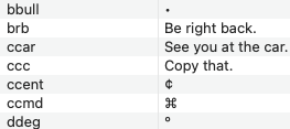
Great idea. Personally I use macOS text replacement: hhalf for ½, ccent for ¢, ttm for ™, ccopy for ©, aapple for , bbull for •, etc.
What struck me was that I use a mixture of these two techniques (OK, I use Typinator instead of the macOS’s text replacement system, but the idea is the same).
For example, like Cabel, I type the bullet (•) and ellipsis (…) characters directly; But like David, I use abbreviations (the Typinator term for text substitutions) for the cent (¢), trademark (™), and apple () symbols. Is there any logic to my system?
Certainly, some symbols that I use fairly frequently, like ⌘, ⌥, ⇧, and ⌃, have to be handled by abbreviations because they can’t be typed directly using the Option or Option-Shift keys.


But as you can see, the and ¢ characters can be typed directly. So why don’t I? I guess it comes down to habit. Long, long ago—back in the 80s, before the Mac had text substitutions or abbreviation utilities—I learned how to type certain characters using Option and Option-Shift because I needed them and there was no other way to get them. So bullet (•), degree (°), ellipsis (…), the n- and m-dashes (– and —), and all the curly quotation marks (‘,’,“, and ”) became part of my muscle memory—muscle memory that was somehow retained even after I took an eight-year Mac hiatus in the late 90s and early 00s.
But I never needed ™, ©, or enough to train my fingers how to type them. When I returned to the Mac and started using text expansion utilities,2 these were among the special characters I created abbreviations for. Expansion made it unnecessary to learn new key combinations.
There is one special character I’ve recently learned to type directly: Δ. I use this character to delimit equations here on the blog. I wanted something that was easy to type (⌥J) and had a mathy feel to it. So when I want to show something like
I type
ΔΔ \int_0^a \sin x \, d x ΔΔFor inline equations I use a single Δ.
I have a feeling many longtime Mac users are like me: some special characters are typed directly, some are done through expansion, and the rest—never used before and never expected to be used again—come through the Character Viewer.

-
Since Twitter is now X, I feel “tweet” has fallen into the public domain and can be applied to any shortform social media system. ↩
-
I’ve used TypeIt4Me, TextExpander (originally as Textpander), and now Typinator. ↩