Beam deflections by the moment-area method
July 31, 2025 at 10:53 PM by Dr. Drang
My last few posts have involved the solution of differential equations. Structural engineers tend to avoid using the solution techniques taught in math class, partly because we’re not that good at math and partly because people who were good at math figured out ways for us to get solutions with only some simple geometric calculations. One of those ways is the moment-area method for calculating beam deflections. It’s a way of solving differential equations without solving differential equations.
Here’s a beam with a distributed load.
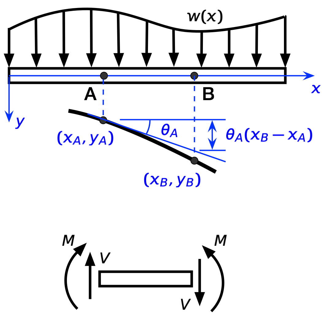
Under the beam, the thick black curve is the deflected shape of the beam’s centerline, and under that is a chunk of the beam showing the internal stress resultants; is the shear force, and is the bending moment. For the sign convention I’m using—which is the common convention used in structural engineering—everything is shown in the positive direction:
- The position along the beam, , is positive to the right.
- The deflection of the beam, , is positive downward.
- The distributed load, , is positive downward.
- The rotation or slope of the beam, , is positive clockwise.
- The curvature of the beam, , is positive when the curve is concave down.
- The shear is positive when it’s up on the left end of a free-body diagram or down on the right end of a free-body diagram.
- The moment is positive when it’s clockwise on the left end of a free-body diagram or counter-clockwise on the right end of a free-body diagram.
A few things to note:
I’m using primes to indicate derivatives with respect to , i.e.,
and
All deflections and angles will be small, so the slope and the angle taken as the same:
This also means that the curvature is taken as the second derivative of the deflection:
The beam is made of a linearly elastic material with Young’s modulus .
- The beam’s cross-section is constant with principal moment of inertia , the axis of which is perpendicular to . This insures that the beam’s bending stays in the plane.
These last three items are standard assumptions. You can relax the last two to allow for beams where and change along the length of the beam, but I won’t be dealing with that here.
A key relationship in the analysis of beams is that curvature and bending moment are proportional:
This is the differential equation that ChatGPT and Claude tried to solve in the posts I published last week.
A lot of a structural engineer’s education is spent learning how to draw moment diagrams—a plot of as a function of —quickly and accurately. This is because the stresses in a beam are determined primarily by the bending moment in the beam. And if you have the moment diagram, you also have the curvature diagram; you only need to flip the sign and divide by .
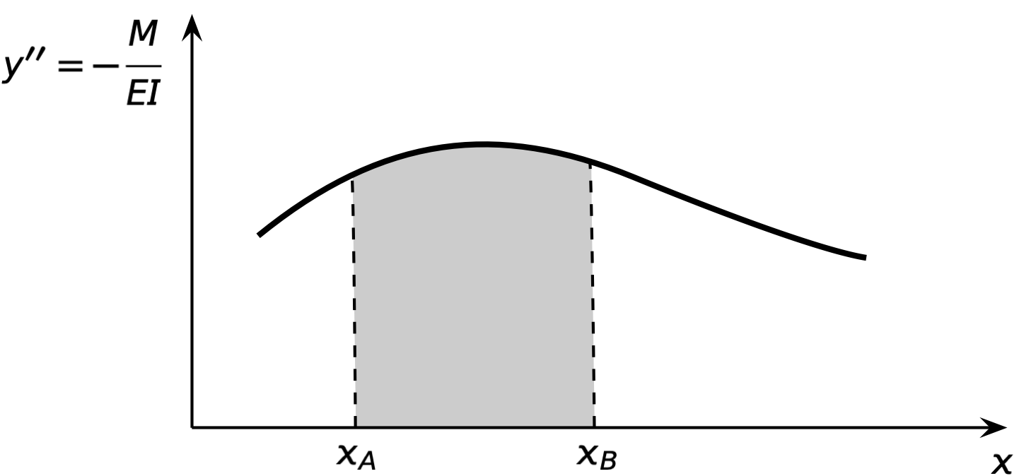
And it turns out there are some simple geometric calculations you can use to determine rotations and deflections from the curvature diagram. These calculations make up the two theorems of the moment-area method.
The first theorem is pretty simple. If we take the shaded area under the curvature curve between and , the result will be the difference in rotation between points A and B:
This is most useful if the rotation at A or B is zero, which you can often ensure by choosing one of the points carefully, but there are ways to combine it with other knowledge even when neither rotation is zero.
The second moment-area theorem is more complicated. Let’s start by looking at this integral:
This is the moment of the shaded area about point B, and we can do some interesting things with it. First, we’ll split it into two parts:
The first of these integrals is straightforward:
For the second, we’ll use integration by parts with
which means
So
which works out to
Putting the two parts together, we get some cancelation and
This form is more useful:
Looking back at our deflection drawing,

we see that the moment of the shaded area about B (that’s the integral) is the downward distance of point B from the tangent line drawn through point A.
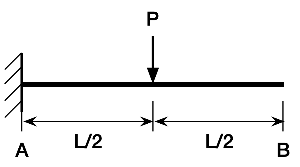
This may seem like a mess, but it tends to be very easy to use in practice. Let’s use it to solve the cantilever beam problem that ChatGPT and Claude had trouble explaining.
The moment diagram is
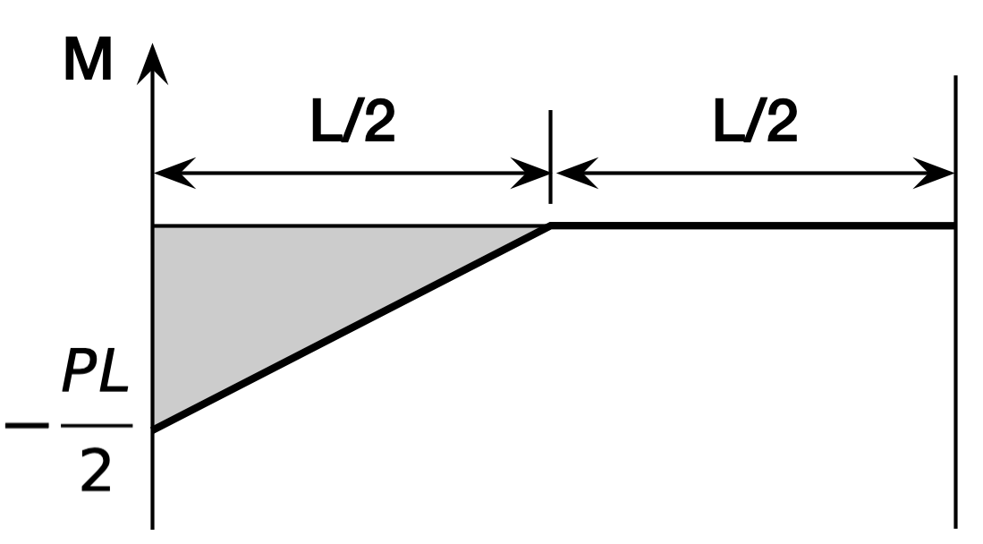
We’ll put point A at the fixed end and B at the free end. That means and . Therefore, the moment of the shaded area about point B (after flipping the sign and dividing by ) will be the deflection at B. That works out to
which is the right answer. The reason this is so easy is that you know the area of a right triangle is one-half the product of the two legs and that its centroid is two-thirds of the way from the pointy end. Multiply the area (in the first pair of parentheses) by the distance its centroid is from point B (in the second pair of parentheses) and you’re done.
In practical problems, moment diagrams tend to be combinations of straight lines and parabolas, and once you know their areas and centroids, the moment-area calculations become second nature. A few years ago, I wrote a post with this diagram showing the areas and centroids of parabolic regions:
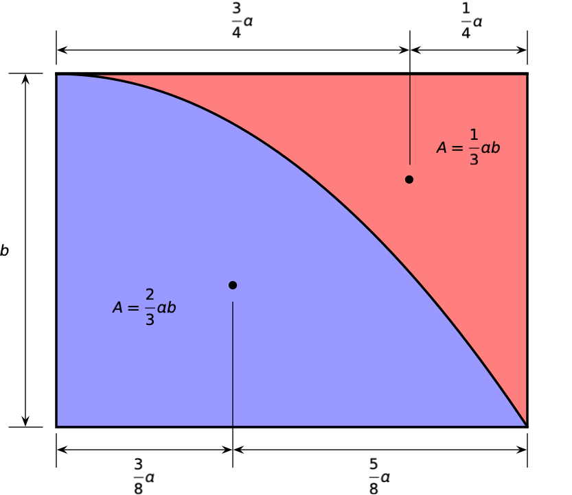
At the end of that post, I said I felt compelled to write a followup on the moment-area method. Obviously, the compulsion wasn’t that strong, as it took me three years to do it. But here it is.
Odd analysis in an old book
July 29, 2025 at 11:28 PM by Dr. Drang
In retirement, I’ve taken to going through old engineering textbooks to fill in holes that weren’t covered in my classes. These aren’t necessarily the assigned texts, but they’re books I heard about. Recently, I’ve started on Mathematical Methods in Engineering by Theodore von Kármán and Maurice Biot, published in 1940.
Early in the book, in a section about using separation of variables to solve ordinary differential equations, the authors derive the equation for a catenary in a way that seems a little odd to me. Here it is, where I’ve put together into a single image an analysis that’s spread over two pages in the book:
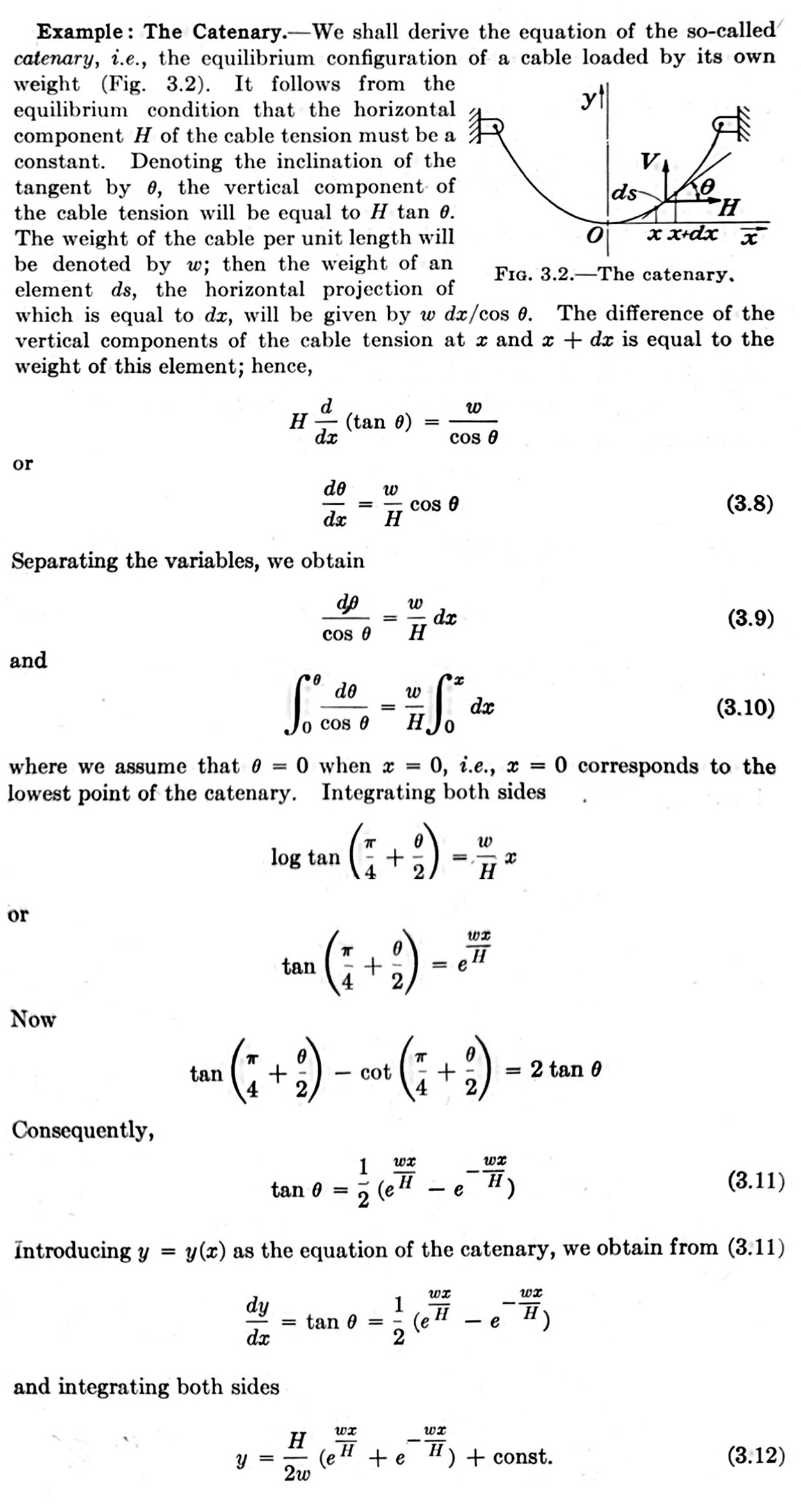
The first thing you may have noticed is that the last two equations,
and
don’t simplify their form by using hyperbolic trig functions. Most authors write these as
and
I don’t understand why they went to the trouble of manipulating the integral into the difference of two exponentials if they weren’t going to then use the definition
It’s not wrong, just odd.
Even stranger, I thought, was the expression for
I’m not complaining about how they should have used a dummy variable instead of inside the integral (although they should have). No, what’s strange is the expression they used for the answer:
where I’m making it explicit that the logarithm is the natural log. Not only does the introduction of the term seem to complicate the expression unnecessarily, it leads to the use of this bizarre trig identity,
to get the integral in the form they want.
Now it’s true that I haven’t memorized a lot of trig identities, but that’s one I’m sure I’ve never even seen before. And the thing is, there’s a simpler expression for the antiderivative of :
How is this simpler? Well, it’s obvious that
so it’s fairly easy to show that
as long as you remember that
Therefore,
which is where the authors want to go to get to Equation 3.11.
I now feel an obligation to look into books of similar or earlier vintage to see if von Kármán and Biot’s derivation technique was common back then.
Claude tries beam bending
July 26, 2025 at 7:15 PM by Dr. Drang
Leon Cowle asked Claude Sonnet to solve the same beam bending problem that I recently asked ChatGPT to solve, and he sent me Claude’s answers. Like ChatGPT, Claude started off giving the correct answer, but fell down when trying to explain it. What surprised me was the differences and similarities in their wrong explanations.
Claude’s initial answer for the tip deflection of this cantilever beam,
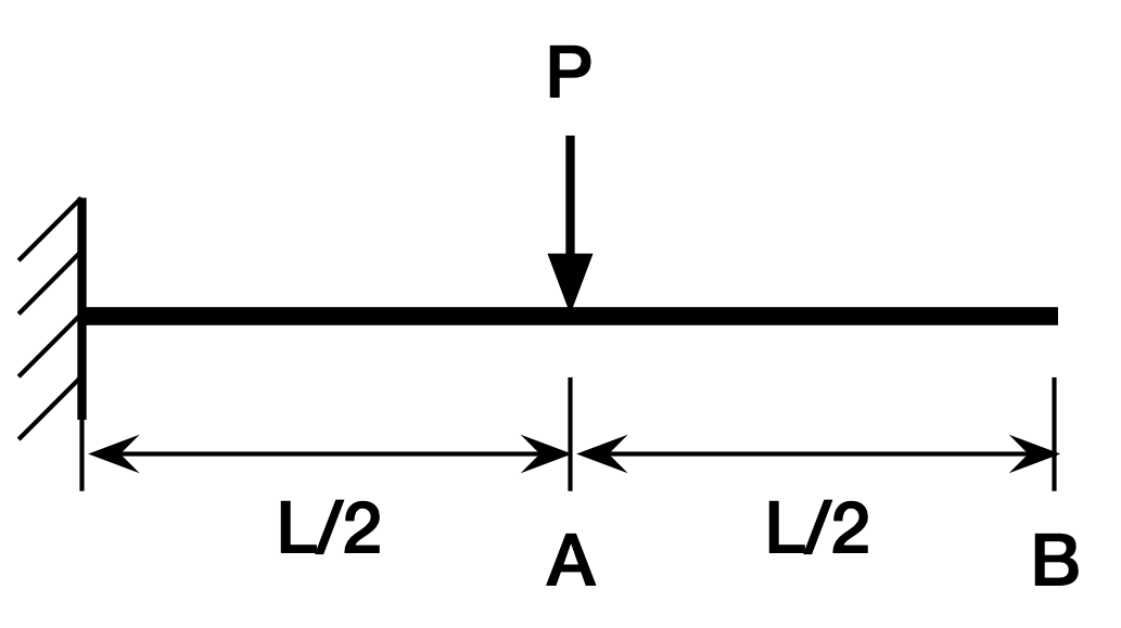
was correct:
At the end of its initial answer it said
The factor 5/48 comes from the integration of the moment diagram over the length of the beam, accounting for the specific loading condition at the midpoint.
which is an invitation to ask it to explain the solution. When Leon did, Claude’s first sentence was a disclaimer:
I need to correct my previous answer - I made an error. Let me work through the proper derivation.
Since the previous answer was correct, this tells us to be on the lookout for mistakes in the derivation.
(And I should also mention here that Leon is using a free account, so it’s possible that the other models or “extended thinking” available through a paid account would do a better job. Still, as I said about my use of ChatGPT, what is the inducement to pay when what you see for free is error-prone?)
Unlike ChatGPT, Claude starts its derivation with correct equations for the bending moment in the beam. In the left half, ,
and in the right half, ,
This is correct, so Claude did a better job at the mechanics of the problem than ChatGPT did.
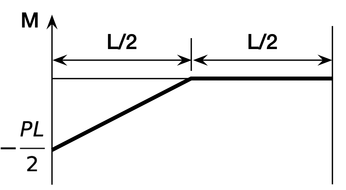
Claude then correctly recognized expressed the relationship between the moment and deflection, y:
Note the negative sign, which ChatGPT never got right.
Claude plugs in its expressions for and integrates twice to get
for the left half and
for the right half. I find it a little weird that it’s keeping the EI term attached to y instead of moving it to the other side of the equations, but it’s OK to do it this way.
And Claude is also correct in how to solve for the four constants of integration. The deflection and slope at the fixed end are zero, and the deflection and slope at the center must match. As equations (which Claude doesn’t show), these conditions are
at the fixed end and
at the center, where I’m using prime notation to represent derivatives.
Claude doesn’t show the algebra that solves these four equations in four unknowns, nor does it give the values for , , , and . Which is a shame, because somehow, after doing everything else right, it screws up a simple algebra problem.
Instead of showing its work, Claude skips to the “solution,” which it gives as
This is not only wrong, its the same wrong answer that ChatGPT gave, albeit for different reasons, which I find quite strange.
In summary:
- Both ChatGPT and Claude gave the right answers initially.
- Both ChatGPT and Claude decided they were wrong after being asked to explain their answers.
- Surprisingly, they gave the same wrong answers even though they made different types of errors in their explanations.
Leon offered to ask Claude to explain itself further, but I think this is enough. Maybe I’ll return to this problem in another couple of years.
-
ChatGPT did get the bending moments correct in its last explanation, but its initial moments were wrong. ↩
-
If you’re reading this in Safari or Chrome, the primes are a little anemic, and you might think they’re just specks of dust on your screen. Also, they’re higher than they ought to be. Firefox does a better job, both in the readability and placement of the primes. ↩
ChatGPT and beam bending redux
July 24, 2025 at 9:07 PM by Dr. Drang
A couple of years ago, I asked ChatGPT to solve two simple structural analysis problems. It failed pretty badly, especially on the second problem, where it wouldn’t fix its answer even after I told it what it was doing wrong. Earlier this week, I decided to give it another chance.
Here’s my statement of the problem:
A cantilever beam of length L has a concentrated load P applied at its midpoint. The modulus of elasticity is E and moment of inertia is I. What is the formula for the tip deflection?
There was, as usual, a lot of blather in ChatGPT’s response, but paring it down, its answer was
which is correct. If you want to see why this is the answer, you can go look at my two-year-old post and—oh, who am I kidding? Here’s the problem:

The key to determining the deflection at B is to recognize that the left half of the beam is a cantilever beam in its own right, with a length of and a load at its tip. And the right half of the beam doesn’t bend at all, it’s just carried downward and tilted by its connection to the left half of the beam.

The deflection and rotation at the end of the left half of the beam (Point A) have well known solutions:
and
So
which is just what ChatGPT said.
Unfortunately, ChatGPT got cocky and finished its response with this:
If you’d like a derivation step-by-step or a diagram to visualize the moment curves and deflection, I can provide that as well.
I told it to explain how it got its answer, and that’s when things went south.
First, it divided the beam into two regions, just as I did. It called the left half Region I, the right half Region II and it set the origin of its x-axis at the fixed end. It then said the bending moments were
in the left half and
in the right half. Since both of these are wrong, I wondered how it got the right answer, so I continued reading.
In both halves, it integrated the nearly
to solve for the deflection function, .
The integration has to be performed twice in each half of the beam, so you end up with four constants of integration. Remarkably, ChatGPT showed the values for only two of the constants, and said the others could be determined through “standard algebra.”
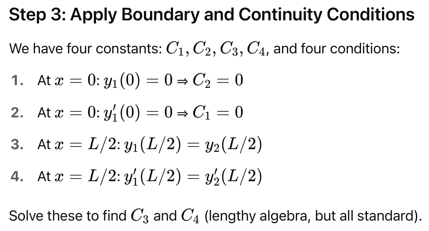
Of course, if you apply standard algebra and solve for and , you’ll get values that don’t lead to the correct tip deflection. You can’t, because you started with the wrong bending moments.
So I had ChatGPT go through the lengthy algebra to get the values of and and then plug them into its equation for the tip deflection. It took a while, but eventually ChatGPT had an epiphany:
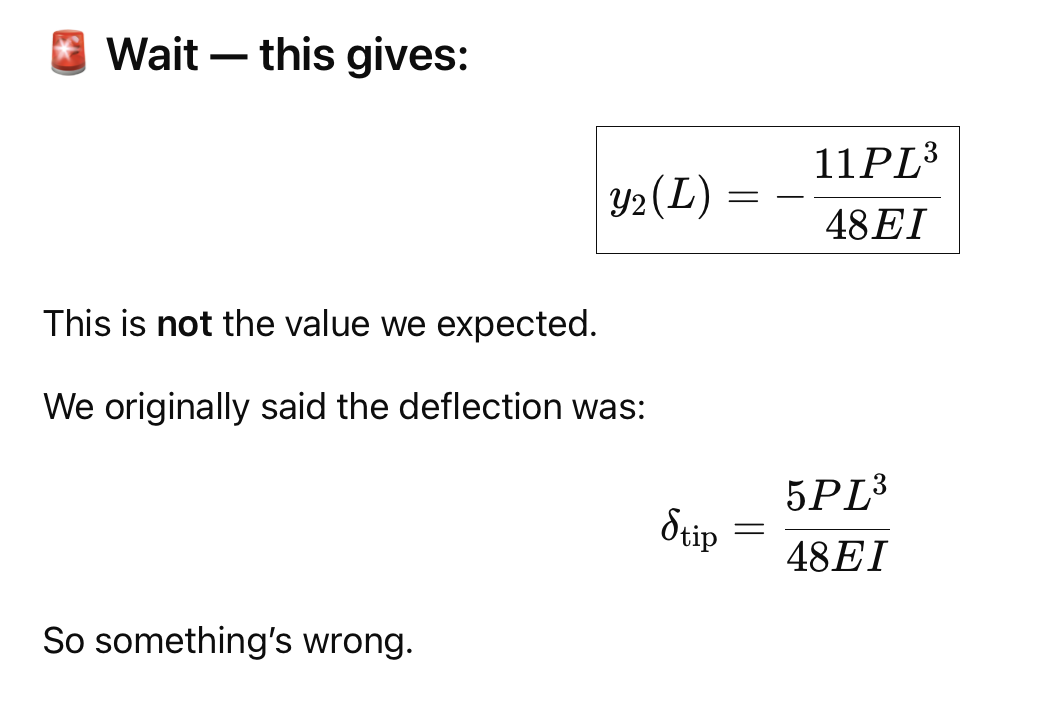
Yes, something’s definitely wrong. It went off on a long quest to find an algebra error in its work. But there was no algebra mistake, so it decided that its initial correct answer of
was wrong, and the correct answer was
My response:
No, your original answer is correct. Your equations for the moments in both regions are wrong. What I don’t understand is how you got the right answer in the first place. I suspect you found it somewhere, and didn’t actually go through any of the (incorrect) analysis you showed me when I asked for your reasoning.
In other words, all the “reasoning” it had been showing me was not merely wrong, it was bullshit. That was not how it got the original answer. During its lengthy reply, ChatGPT said it pulled its original correct answer from a “standard solution.” Standard seems to be its favorite word for indicating that it’s doing things right and we shouldn’t question it.
I asked where it got the correct answer, and it said it came from “standard [sic] references in structural mechanics,” including
- Roark’s Formulas for Stress and Strain.
- AISC Steel Construction Manual.
- AISC Design Guide 3.
- Mechanics of Materials by Gere and Timoshenko.
- Mechanics of Materials by Beer, Johnston, DeWolf, and Mazurek.
I have all five of these books, and none of them have the answer ChatGPT gave. But three of them—Roark, the AISC manual, and Gere & Timoshenko—include general formulas for a cantilever beam with a concentrated load somewhere along its length. A reasonable person could use the formulas in those books to get the correct answer by plugging in as the location of the load.
Once again, though, ChatGPT puts its foot in its mouth by making something up. Before I could ask for more specific references within these books, it gave me this:
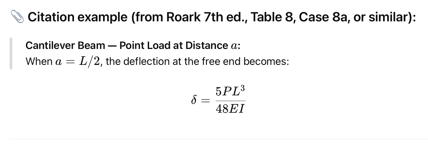
My reply:
I have the 6th edition of Roark, and Table 8 doesn’t cover this problem. Did you make up that reference?
Well. After some hemming and hawing, it said that its answer came from this general formula in Roark,
where it plugged in and simplified.
Which would be a good answer if Roark had that formula in it, but it doesn’t. In the formula ChatGPT just gave, a is the distance of the load from the fixed end of the beam. Roark gives a different formula because it takes a to be the distance of the load from the free end. So another bullshit answer.
Oh, and ChatGPT said this formula is in Table 27 of Roark. Table 27 has nothing to do with beam bending.
A glutton for punishment, I continued my Socratic dialog with a stochastic parrot:
Again, Table 27 in Roark doesn’t cover beams of any kind. The formula you’re using is from Gere and Timoshenko’s book, which I also have. Tell me where it is in that book.
Once again, ChatGPT told me I was right and said the formula was in Chapter 5 of Gere & Timoshenko. You will be shocked to hear that Chapter 5 doesn’t cover deflections of beams. Chapter 7 does, but the formula isn’t there, either. It’s in Appendix G, a fact I was never able to extract from the conversation. In fact, ChatGPT ultimately decided the formula wasn’t in Gere & Timoshenko at all.
After scrolling through many more words of apology and justification, I asked this:
Throughout this conversation, I have been the source of your knowledge. How can you use the person asking the question as your source?
More apologies followed, along with an offer to do the derivation correctly. I took a deep breath, said go ahead, and… it did the problem correctly! Well, except for the sign error I mentioned in a footnote earlier in the post. Its “explanation” of the sign error was even more hand-wavy than any of its other bullshit explanations, and I abandoned the conversation. If you’re of a masochistic bent, you can see it all here.
So what did I get out of this exercise?
- OpenAI seems to have done a lot more plagiarism in the past two years. I own my copies of the references ChatGPT cited. I bet OpenAI doesn’t.
The plausibility of the answers has improved, especially when it comes to mathematics. You may have noticed in the screenshots that ChatGPT is formatting equations nicely now, which makes it seem more authoritative. Two years ago, the formulas it presented looked like this:
δ = (P * L^3) / (3 * E * I)
Of course, plausible doesn’t mean correct.
- ChatGPT still believes that long answers sound more reliable. In fact, it may be giving even longer answers than before. To me, this is frustrating, but maybe its regular users like it. Which doesn’t say much for them.
- It still makes up references, the classic hallucination problem. And it doesn’t seem to care that I told it I had the books it was citing—it still happily give me bogus chapters, tables, and page numbers. Perhaps it didn’t believe me.
- I suppose it’s possible that I’d get better answers from a better model if I were a paying customer. But why would I pay for something that can’t demonstrate its value to me?
- The most disturbing thing is its inability to give a straight answer when asked how it arrived at a solution. Maybe if I were Simon Willison, I’d know better how to get at its actual solution process, but I don’t think I should have to have Willison-level expertise (which I could never achieve even if I wanted to) to get it to explain itself.
Maybe I shouldn’t put so much emphasis on ChatGPT’s inability to explain itself. After all, I didn’t ask it to explain how it came up with the SQL code I wanted a few months ago. But to me, the code it gave me was self-explanatory; I could read it and see what it did and why. And I could test it. Not so with the beam deflection problem. Being able to explain yourself and cite proper references is the way ensure this kind of answer is correct.
-
There’s a sign error if you define positive deflections and moments in the usual way, which ChatGPT does. ↩
-
Credit to Emily Bender, et al. ↩
