Saving links to Tot

July 20, 2025 at 11:03 AM by Dr. Drang

I mentioned on Mastodon how much I enjoyed Myke Hurley’s interview of John Gruber on the most recent episode of Cortex. One part that particularly resonated with me was when Gruber spoke of all the online bookmark managers he’s used over the years and how none of them have stuck. It was like I was listening to myself. So when he said he’s shifted to using a Shortcut that saves the page he’s looking at to a list in Tot, I figured I’d give it a try.

I wrote some Tot Shortcuts last year: one for dictating short notes that includes the date, time and location; and another for cleaning up my shopping lists after a trip to the store. I still use them, and I still like Tot in general as a place to put ephemeral notes. I used Drafts for many years, but never cleared out the old notes; Tot’s seven-note limit forces me to keep temporary text temporary.

I keep the links in the 6th dot. Here’s what it looks like on the Mac:

Tot dot 6 with links

For each link, it saves the date, title, and URL on successive lines. Blank lines separate the entries. It sounds as if Gruber’s system is more sophisticated, with an automation that runs every night to (I think) add a date header that applies to all the links saved on that day. That would make the list more compact, but I’m not going to take that step until I know I’ll actually keep using this system.

What is the system? It’s just this Shortcut, which you can make for yourself or download:

Step	Action	Comment
0		Share Sheet input of web page
1		Get name of page
2		Get URL of page
3		Get today’s date
4		Construct the text
5		Add the text to the end of Tot dot 6

Not much to it, which is why I don’t feel bad about building it, even though my track record for saving links is pretty poor. My goal is to use this only for links to pages I intend to write about and to clear them when the post is written. Tot will help with that by getting crowded quickly.

To make it easy to use this Shortcut, I’ve added it to my favorites. It appears just below Copy in that section of the Share Sheet on both my iPhone and iPad.

Shortcut added to Favorites

Running a Shortcut from the Mac Share Sheet takes more clicking than I’d like, so if I use this enough to get frustrated by the extra work, I’ll probably make a Keyboard Maestro macro that does the same thing.

Cauchy coup

July 19, 2025 at 10:03 PM by Dr. Drang

Bruce Ediger, who blogs at Information Camouflage, has been doing some interesting numerical experimentation recently; first in a post about estimating population size from a sample of serial numbers (you may have seen this Numberphile video on the same topic), and then a couple of videos about the Cauchy distribution. In the first, he looked at the sum of two random variables that are Cauchy distributed; in the second, he looked at the quotient of two normally distributed random variables, which—under certain conditions—is supposed to have a Cauchy distribution.

By numerical experimentation, I mean that Ediger’s generating sets of random numbers, doing some calculations on them, and then seeing how close his calculations are to certain theoretical results. It’s a good way to get a feel for how things work, and it’s the kind of analysis that’s really only possible because of the computational power we all have at our fingertips. This sort of playing around with thousands and thousands of numbers just wasn’t feasible when I was learning probability and statistics, and I’m jealous of today’s students.

What attacted my interest in Ediger’s post on the quotient of two normals was the possibility that I could do the problem analytically without too much effort—mainly because the same computational power that lets him mess around with a hundred thousand quotients of random samples also lets me do calculus and algebra without dropping terms or making other silly errors.

Cauchy from the quotient of two zero-mean normals

I started by making sure I could prove that the quotient of two zero-mean normals has a Cauchy distribution. The analysis in this section follows the structure outlined in Papoulis’s Probability, Random Variables, and Stochastic Processes.

We begin by looking at the general problem of the quotient of two random variables of any distribution. We’ll call the two random variables X and Y and their joint probability density function $f_{X Y} (x, y)$ .

We’ll call our quotient Z and define it this way:

Z = \frac{X}{Y}

To figure out the probability density function of Z, we’ll first look at its cumulative distribution function, $F_{Z} (z)$ , which is defined as the probability that $Z \leq z$ ,

F_{Z} (z) = P (Z \leq z)

This probability will be the volume under the joint PDF of X and Y over the region where $X / Y \leq z$ . That’ll be this integral:

F_{Z} (z) = \iint_{x / y \leq z} f_{X Y} (x, y) d x d y

And the domain over which we take the integral will be the blue region in this graph,

Quotient integration domain

where the region extends as far as $f_{X Y} (x, y)$ extends in the upper left and lower right directions.

If this doesn’t seem obvious to you, don’t worry, it isn’t. But think of it this way:

If $y > 0$ , then $x / y$ will be less than $z$ when $x$ is to the left of the $x = z y$ line.
If $y < 0$ , then $x / y$ will be less than $z$ when $x$ is to the right of the $x = z y$ line. Making $y$ negative flips the direction of the less-than sign.

With the integration domain defined, we can write the expression for $F_{Z} (z)$ like this:

F_{Z} (z) = \int_{0}^{\infty} \int_{- \infty}^{z y} f_{X Y} (x, y) d x d y + \int_{- \infty}^{0} \int_{z y}^{\infty} f_{X Y} (x, y) d x d y

To get the PDF of Z, we need to differentiate $F_{Z} (z)$ with respect to z. This is done through the Leibniz rule. Normally that would leave us with six terms, three for each of the two integrals above. But luckily for us, four of those terms are zero, leaving

f_{Z} (z) = \int_{0}^{\infty} y f_{X Y} (z y, y) d y - \int_{- \infty}^{0} y f_{X Y} (z y, y) d y

Now it’s time to consider the case when X and Y are jointly normal. And to get to a Cauchy distribution for Z, both X and Y will have to have zero means. With that restriction, the joint density function will look something like this:

Joint normal surface plot

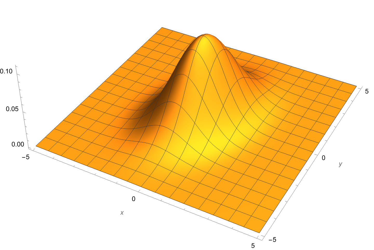
To make the plot, I needed some actual numbers, so I’ve given X a standard deviation of 1, Y a standard deviation of 1.5, and the correlation coefficient a value of 0.25. The analysis doesn’t rely on these or any other particular values for the parameters.

We can see the joint PDF’s structure a little better with a contour plot:

Joint normal contour plot

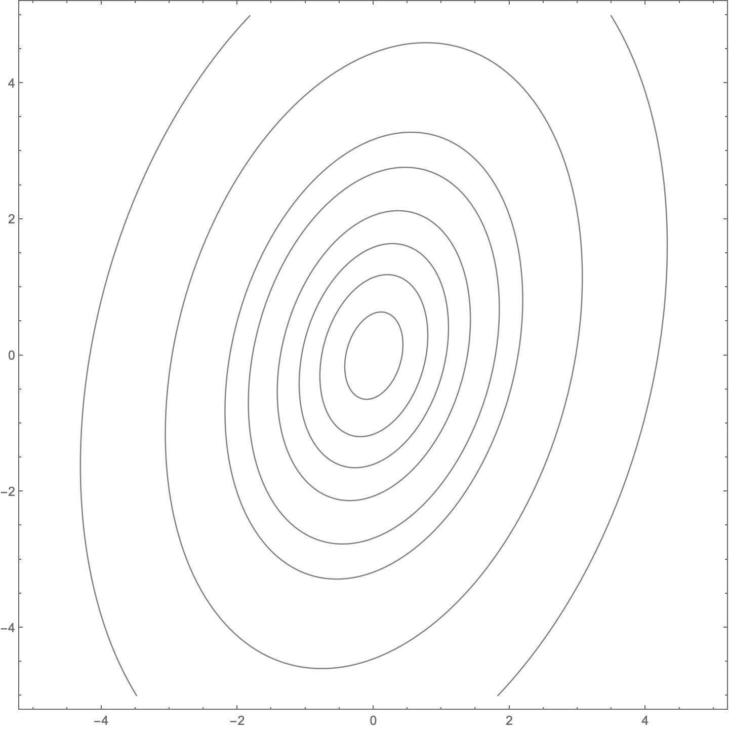
The key is that it has this kind of symmetry,

f_{X Y} (x, y) = f_{X Y} (- x, - y)

and we can take advantage of that symmetry to simplify the expression for $f_{Z} (z)$ :

f_{Z} (z) = 2 \int_{0}^{\infty} y f_{X Y} (z y, y) d y

OK, now we have to get into the nitty gritty and actually do some integration. Which means it’s time to abandon “by hand” analysis and switch to Mathematica. Here’s the notebook that does the following:

The integration to determine the form of $f_{Z} (z)$ . When writing stuff like this by hand, I would typically use $σ_{X}$ , $σ_{Y}$ , and $ρ$ for the standard deviations of X and Y and their correlation coefficient, but to make the typing easier in Mathematica, I use sx, sy, and r.
Checks the result against Papoulis’s. It’s not uncommon for Mathematica to give answers that don’t look like what you’ll find in a book, even though they are algebraically equivalent.
Determines the shape and location factors, $γ$ and $z_{0}$ , that put the result into the generic form for a Cauchy distribution that we see in the Wikipedia article:
$f_{Z} (z) = \frac{γ}{π [(z - z_{0})^{2} + γ^{2}]}$

Here’s the notebook:

So yes, the quotient of two zero-mean normals has a Cauchy distribution with a shape parameter of

γ = \frac{\sqrt{1 - ρ^{2}} σ_{X}}{σ_{Y}}

and a location parameter of

z_{0} = \frac{ρ σ_{X}}{σ_{Y}}

Ediger’s problem

That was sort of a warmup to make sure I understood how to use the MultinormalDistribution function. It’s time to move on to Ediger’s problem.

Ediger doesn’t take the quotient of two zero-mean normals. Instead, he takes the quotient of two independent ( $ρ = 0$ ) normals, one with zero mean and unit standard deviation, and the other with a mean of 1 and standard deviation of 3. This shouldn’t result in a Cauchy distribution, and it doesn’t. But to see how close it is, I made this Mathematica notebook:

Comparing the actual distribution of the quotient (in blue) with Ediger’s best fit of a Cauchy distribution (orange), we see this:

Exact PDF vs Ediger fit

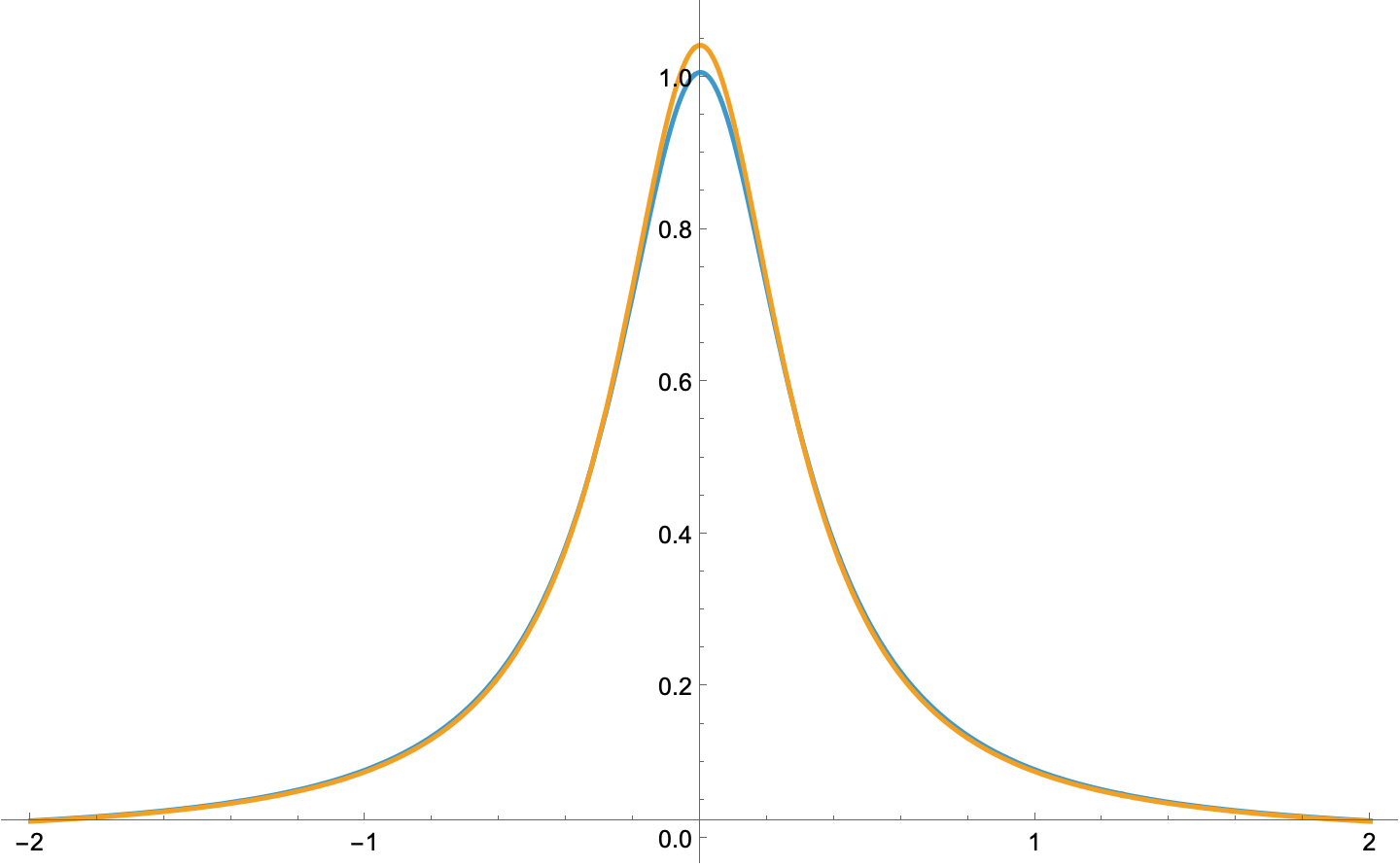
Definitely not the same but pretty damned close.

Finally

I’m not sure most people would consider this recreational mathematics, but it’s recreational to me. You should see the things in my notebooks that don’t get turned into blog posts.

A habit I picked up from my thesis advisor is to use capital letters for random variables and their lower case versions for particular instances of those random variables. ↩

Settings steganography

July 16, 2025 at 12:10 PM by Dr. Drang

Last week, I was going to be out with my MacBook Pro all day, and I wanted to make sure it was fully charged. I had noticed that it was typically charging up only to about 80%, and I assumed that was because Sequoia was doing some clever battery-life-lengthening thing. I wanted to turn the clever thing off so I could get the battery to 100% just for that day.

You will probably not be shocked to hear that I didn’t find the solution by simply opening System Settings and scanning the Battery panel—I had to do a Kagi search for it. It wasn’t that the toggle was buried several layers deep or that it was outside the Battery hierarchy. No, the problem was that Apple had put the toggle in a place where toggles—or any kind of control or data entry field—don’t belong.

Here’s the Battery settings panel:

Battery panel in System Settings

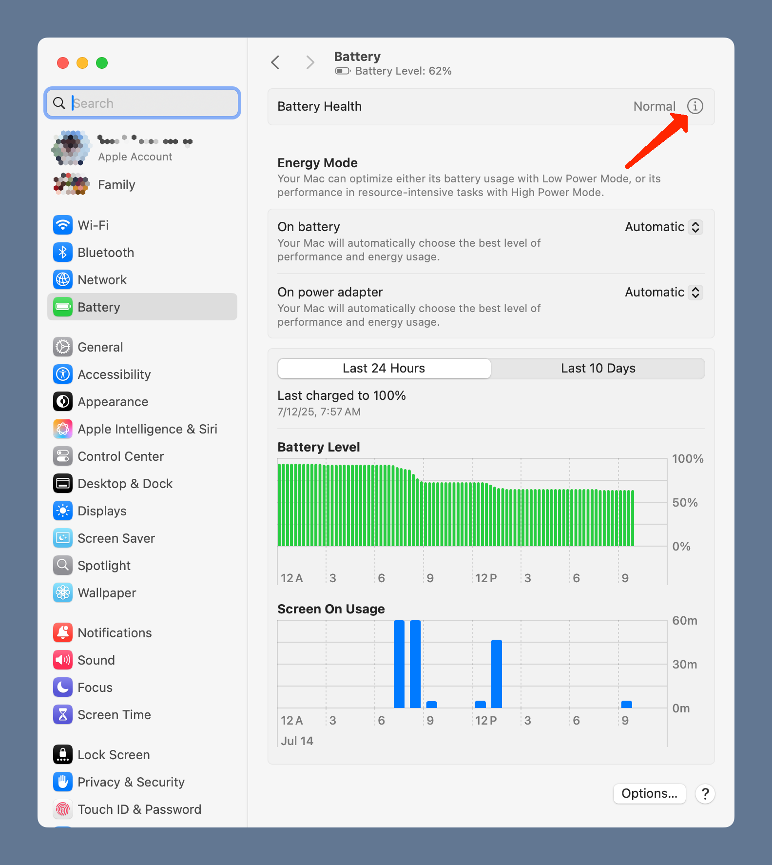
The two popup menus in the Energy Mode section of the panel aren’t what I wanted, so I assumed the setting for turning off battery optimization would be found via the Options… button down at the bottom of the panel. But it wasn’t in the window that appeared when I clicked it.

Battery options window

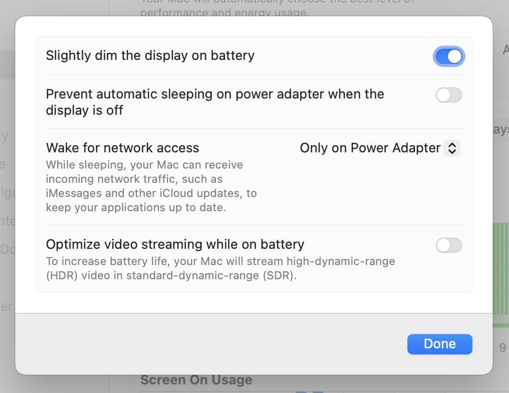
Well, I’ve already given away the secret with the red arrow in the first screenshot. You have to click the ⓘ button near the top right corner. That brings up this window with the toggle I was looking for.

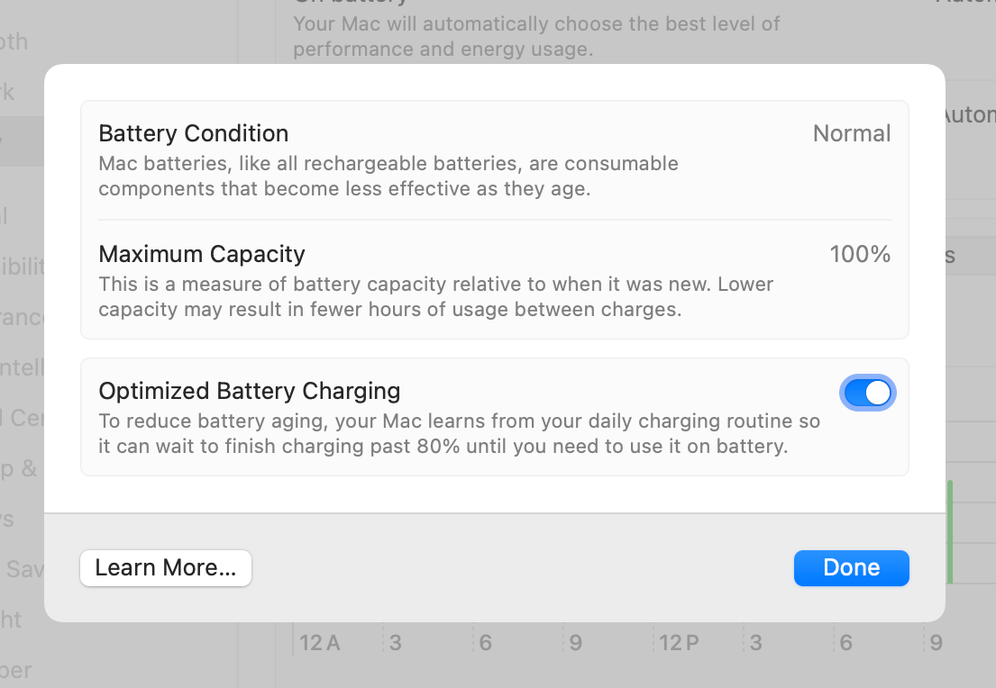
Battery info window with optimized charging toggle

Turning the toggle off brought up this further set of options:

Optimized battery charging options

Before I start complaining, let me say this final dialog box is nice. You can turn off optimized charging permanently if you want, but the default is to just turn it off for a day. The clear implication is that Apple thinks you should use non-optimized charging rarely, and it will help you turn it back on tomorrow if you forget.

Now for the complaint: none of this should be behind the ⓘ button. The “i” clearly means “information,” and when I click on it, I expect to be given information, not to give it. Just as you wouldn’t put toggles or other controls behind the ?⃝ button, you shouldn’t put them behind the ⓘ.

I know there’s always talk of Apple losing its way in user interface design. And that talk has been especially loud since the release of the xxxOS 26 betas. My Mastodon timeline has been filled with criticism of Liquid Glass and Alan Dye for weeks, and it’s tiresome to read the constant grousing. But then I run into this, and I need to do some grousing myself.

When Venus is in the House of Games

July 7, 2025 at 1:01 PM by Dr. Drang

I had a touch of insomnia last night and tried to cure it by watching YouTube videos. The algorithm suggested a compilation of quiz questions from Richard Osman’s House of Games, a British game show that I used to watch regularly back in 2020, when I was trying to take my mind off of things I had no control over.

The cure didn’t work, because the video I watched was this one, and the last question—which starts at about the 26:35 mark—gave what I was sure was the wrong answer. So instead of falling asleep, I went off to look up the right answer and then got caught up in how to calculate it.

The question was “How many hours are there in one day on the planet Venus?” and the answer they gave was 5,832. Now, I am by no means an expert on Venusian planetary motion. I know its year is somewhat more than 200 Earth days, that it rotates backwards, and that its days are quite long. But in my mind, “quite long” is nowhere near 5,832 hours.

So I went to NASA’s Venus Fact Sheet, which told me that its day is 2,802 hours, roughly half of what House of Games said. But the number 5,832 did appear in the section on Venus’s orbital parameters:

Orbital parameters for Venus

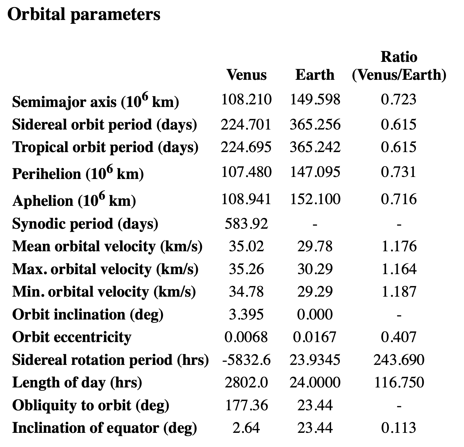
It’s fourth from the bottom in the row labeled Sidereal rotation period. I took the negative sign to be an indication of Venus’s backward rotation, similar to the obliquity being given as 177.36° instead of 2.64°.

(By “backward rotation” I mean that Venus rotates in the opposite direction of its revolution around the Sun.)

So now I felt compelled to figure out how the -5,832.6 hours of sidereal rotation related to the day length of 2,802.0 hours. Which kept me awake longer.

First, I noticed—or rather, PCalc told me—that the sidereal orbital period of 224.701 Earth days is 5392.824 hours, a number that’s fairly close (in magnitude) to the sidereal rotation period. I imagined looking “down” on a solar system in which a planet revolved counter-clockwise around its sun and rotated clockwise about its axis at the same speed. It would look like this at various points in its year:

Backward rotating planet

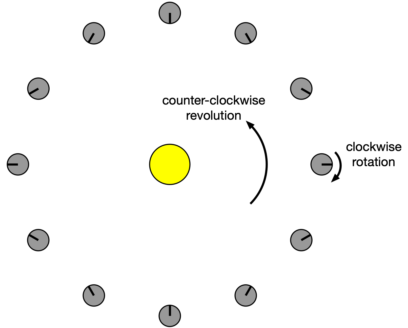
The black line on the planet is a meridional stripe that runs from pole to pole to help see the rotation. For every 30° of counter-clockwise revolution of the planet about its sun, there is 30° of clockwise rotation about its axis. This is all relative to us, who are looking at this from the point of view of the stars (sidereal).

As you can see, midnight to midnight on the planet’s meridional stripe takes half a year. That’s going from the 3:00 position around to the 9:00 position. So for these conditions—a planet rotating clockwise at the same speed it revolves counter-clockwise—there will be two days in a year.

So in rough numbers, there are two Venusian days in a Venusian year. With a Venusian year being about 5,400 hours, that makes its day about 2,700 hours long. But let’s do a more precise calculation to see if we can get all the numbers in the fact sheet to line up.

Taking Venus to move in a circular orbit, its orbital speed is

\frac{360 d e g}{5392.824 h r} = 0.066755 d e g / h r (C C W)

Its rotational speed about its axis is

\frac{360 d e g}{5832.6 h r} = 0.061722 d e g / h r (C W)

So Venus will have gone through one day when

(0.066755 d e g / h r) t = 360 d e g - (0.061722 d e g / h r) t

That works out to

(0.128477 d e g / h r) t = 360 d e g

t = 2802.0 h r s

which matches the value in the table.

This correct answer, by the way, would not have changed who got the points in the game. Both teams were orders of magnitude too low. And with my curiosity satisfied and my phone turned off, I went back to sleep.

And now it’s all this

I just said what I said and it was wrong
Or was taken wrong

Saving links to Tot

Cauchy coup

Cauchy from the quotient of two zero-mean normals

Ediger’s problem

Finally

Settings steganography

When Venus is in the House of Games

Site search

Meta

Recent posts

Credits

And now it’s all this

I just said what I said and it was wrong Or was taken wrong

Saving links to Tot

Cauchy coup

Cauchy from the quotient of two zero-mean normals

Ediger’s problem

Finally

Settings steganography

When Venus is in the House of Games

Site search

Meta

Recent posts

Credits

I just said what I said and it was wrong
Or was taken wrong