The Michelson Fourier Analyzer

January 1, 2015 at 12:31 PM by Dr. Drang

Let’s start the new year off with a bit of Fourier analysis, shall we?

A couple of months ago, Bill Hammack, the YouTube Engineer Guy (and professor of chemical engineering at the University of Illinois) produced a wonderful series of four videos—and a book—about a 19th century mechanical device that does Fourier analysis and synthesis. Here’s the introductory video:

Professor Hammack is always entertaining and informative, but he really outdoes himself in these videos. You can see how delighted he is to have brought this device back to life and show it to us. And why not? It’s a beautiful machine, both in concept and in execution. Like Hammack, I’m a sucker for mechanical devices that perform functions we now think of as exclusively digital.

The machine was designed by Albert Michelson (of the Michelson-Morley experiment) near the turn of the 20th century while he was at the University of Chicago, and it was built by William Gaertner & Co., a local Chicago firm. It currently sits in Illinois’s Altgeld Hall, just across the Quad from Professor Hammack’s office.

Altgeld Hall is known to all Illinois grads as the building with the bell tower that chimes on the quarter-hour and serenades the north half of campus with carillon music. It’s the home of the math department and a little post office with appropriate postmarks. It also houses the math library, my favorite library on campus. It covers two stories in the middle of the building and has lovely old cast iron shelves and a glass block floor set in an iron grillage. Everything about it, including the musty smell, says “library.”

As it happens, just a month before Hammack published the videos, I was in Altgeld Hall with my older son. We were there for a campus visit, and I took him through Altgeld to show him the library and the collection of mathematical models that line several of the halls. In one of the halls, sitting almost anonymously in a glass case, was Michelson’s Fourier Analyzer. I read the descriptive card inside the case but didn’t believe it was in working order.

Before talking about the Analyzer, let’s review what Fourier analysis is and why we use it. Periodic functions appear in the mathematical solution to many problems of practical physical importance. The simplest periodic functions to calculate with are sines and cosines, and as it turns out, any periodic function can be expressed as a series of sines and cosines:

f (x) = a_{0} + \sum_{n = 1}^{\infty} a_{n} \cos (n x) + \sum_{n = 1}^{\infty} b_{n} \sin (n x)

Joseph Fourier was the first to recognize the value of this series in the solution of the partial differential heat equation, and it’s named in his honor. The trick of Fourier analysis is figuring out the as and bs that make the best fit to the original function, f.

As an example, let’s look at a triangular wave function.

Because the triangle is an odd function, $f (- x) = - f (x)$ , all the cosine coefficients are zero. And because each half-wave is symmetric, the even sine coefficients are also zero. The Fourier series for the triangular wave is then

\frac{8}{π^{2}} [\sin (x) - \frac{1}{9} \sin (3 x) + \frac{1}{25} \sin (5 x) - \frac{1}{49} \sin (7 x) + \dots]

I’ll spare you the math necessary to determine the coefficients. If you’re interested, take a look at equations 7, 8, and 9 in the MathWorld article.

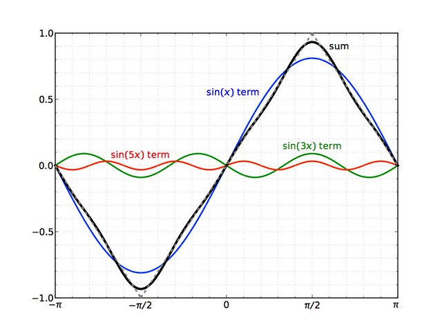
Here are the first three component functions (in blue, green, and red) and their summation (in black):

You can see that even after only three terms, we have a pretty good approximation to the original function, except near the corners at $π / 2$ and $- π / 2$ . Cusps and discontinuities are always troublesome for Fourier series because it’s hard to make smooth functions like sines and cosines fit into sharp corners. This is an example of the Gibbs Phenomenon.

The clearest brief overview of how Michelson’s machine puts together a Fourier series comes in this segment from the Synthesis video:

There are fuller explanations of each component later in the videos, but I think it’s worth mentioning a few things here:

You’ll note that Hammack is showing only the cosine terms of the Fourier series. The Analyzer can do either a sine series for odd functions or a cosine series for even functions, but it can’t do a mixture of sines and cosines for general functions. This isn’t as big a restriction as you might think. Because any function can be split into the sum of an even function and an odd function, the Analyzer can do each part separately, and the user can put the two series together afterwards.
Similarly, the Analyzer doesn’t do the constant term, $a_{0}$ . Since the constant term is nothing more than a vertical shift of the function, this can be removed from the function before analysis and put back in afterwards
The summation goes to 20 instead of ∞ because it’s limited by the number of gears in the machine. If you try to build one with an infinite number of gears, you run out of brass. The Analyzer in Altgeld Hall has 20 gears, but there was an Analyzer Plus that had 80 gears.

Most of the Analyzer’s components work through kinematics. The crank turns through an angle, which causes the set of gears fixed to it to turn through that same angle. Each one of the second set of gears, though, turns through a different angle, based on its diameter and number of teeth. The arms then move through distances according to the angular motion of the gear and cam they’re connected to. This is a complicated dance because of the number of parts, but conceptually it’s fairly simple.

To me, the hardest part to understand is how the movements of the individual arms are added together to drive the up-and-down motion of the pen. I thought Hammack’s explanation of this part was a little hand-wavy, even in the more detailed explanation later in the videos. So I started sketching things out and realized that the addition is done through the assistance of our old friend, Hooke’s Law.

We have a set of parallel arm movements of varying amplitude that we need to add together. The problem is that parallel displacements aren’t additive. If you and a friend start at the same spot, and you walk a mile and she walks two miles, nothing goes three miles. But parallel forces are additive, so if we can convert the displacement of the arms into forces, we’ll be good to go. Converting displacement into force is what Hooke’s Law does.

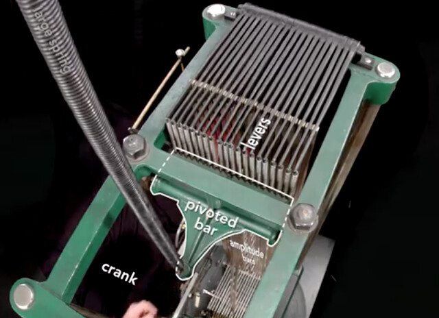
At the top of the Analyzer is a pivoted bar, one side of which is connected via springs to each of levers driven by the individual gears. Here’s a screenshot from the video,

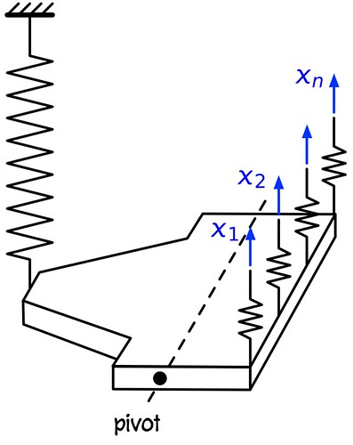
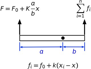
and here’s a simplified sketch of the arrangement,

Forgive me for not drawing in all 20 springs.

The top end of each spring on the right moves a different amount, and the force in each spring will be proportional to that motion. These forces add together into a resultant force on the right that’s balanced, through the lever arms a and b, by the force in the big spring on the left.

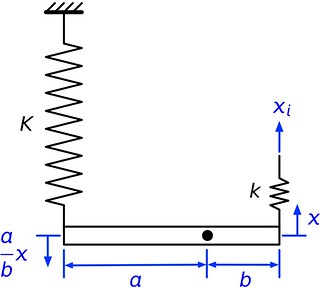
We’ll take $x = 0$ as the position where the bar is horizontal. Because the springs are not in their natural, unstretched state at $x = 0$ , there’s a preload in each spring that has to be accounted for. We’ll call that preload $F_{0}$ for the big spring and $f_{0}$ for the little springs. Here’s the free-body diagram of the pivoted bar:

The equilibrium equation for moments about the pivot leads to

F a = (\sum_{i = 1}^{n} f_{i}) b

(F_{0} + K \frac{a}{b} x) a = (\sum_{i = 1}^{n} [f_{0} + k (x_{i} - x)]) b

where the $x_{i}$ are the displacements of the upper ends of the springs on the right. Rearranging, we get

F_{0} a - n f_{0} b + (K \frac{a^{2}}{b} - n k b) x = k b \sum_{i = 1}^{n} x_{i}

Because the bar is in equilibrium when $x = 0$ and all the $x_{i} = 0$ , the first two terms on the left side cancel, and we can solve for $x$ :

x = \frac{{k b}^{2}}{{K a}^{2} - {n k b}^{2}} \sum_{i = 1}^{n} x_{i}

What this means is that the movement of the pivoted bar, $x$ , is proportional to the sum of the movements of the individual levers, $\sum_{i = 1}^{n} x_{i}$ . The pen is driven by a mechanism attached to the pivoted bar, so its movement is then also proportional to the sum of the movements of the individual levers. This is exactly what we need to add up the terms in the Fourier series. A beautiful solution to the addition problem.

Robert Frost said that writing free verse is like playing tennis without a net. Art needs constraints. I would never want to go back to a time when this was the fastest way to do Fourier analysis, but there’s an artistry to this machine that just isn’t there when you call a routine from an FFT library.

Update 1/4/15 4:08 PM
Theo Honohan pointed out to me in an email that the whippletree mechanism can be used as a displacement adder, and he’s absolutely right. I tend to think of the whippletree as a way of distributing a force uniformly (I’ve used it as such when doing load testing of structures), but it can be used “backwards” to add displacements. It’s probably easiest to think of the whippletree as a way to average displacements, but since the average is just a scaled sum, it works as an adder, too.

I don’t know for sure why Michelson chose to use springs instead of a whippletree, but my guess is that he found the spring system to be simpler and more compact. Whippletrees grow quickly in size as you include more terms in the summation.

If you’re interested in learning about the use of linkages in analog computing, this page by Andries de Man is a good place to start.

And now it’s all this

I just said what I said and it was wrong
Or was taken wrong

The Michelson Fourier Analyzer

Site search

Meta

Recent posts

Credits

And now it’s all this

I just said what I said and it was wrong Or was taken wrong

The Michelson Fourier Analyzer

Site search

Meta

Recent posts

Credits

I just said what I said and it was wrong
Or was taken wrong